TP Physique1
Topic outline
-
-
GENERAL RECOMMENDATIONS
1- ORGANISATION
- A physics (mechanics) practical work TP is scheduled once a fortnight for each group.
- The TP are performed in ascending order. Example: a student who does TP n°3 in the first session will do TP n°4 in the following session.
- Any justified absence will be made up for in a catch-up session scheduled by the same teacher.
- The vice-dean of pedagogy must approve the justification within 48 hours following the absence.
-In case of delay in submitting the justification to the responsible of the matter (more than a week after the absence), the student will have a zero.
- Any unjustified absence will be penalized with a zero.
2- DISCIPLINE IN THE LABORATORY :
A student who comes to physics laboratory must:
- Behaves as a respectful and conscientious student.
- Comes on time (no delay) to the practical session.
- Puts on a white apron.
- Stores stools under benches before going out.
- Has prepared his manipulations (students will be questioned and marked accordingly).
- Brings a scientific calculator and the necessary equipment to draw graphs (pencil, eraser, 30cm ruler, millimeter sheets, etc.), no exchange of equipment (calculator, pencils, etc.) between students will be tolerated.
- The use of the mobile phone is strictly prohibited even to use it as a calculator.
3- REPORTS :
- The practical work session is reserved for the manipulation and exploitation of the results.
- The curves must be drawn in pencil on an entire graph sheet (millimeter paper).
- Reports should be :
a- Written, properly, on practical work sheets provided by the teacher.
b- Given individually to the teacher at the end of the session.
The responsible teachers will provide the marks to students fifteen (15) days after the submission of the reports.
-
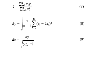
Reminder on the linear regression method
We use the linear regression method only when the absolute uncertainty on x is negligible (Δx ≈ 0) and the absolute uncertainty on y is constant .
This method consists in drawing the best possible straight line of equation y=a+bx which passes as close as possible to all the experimental points, as illustrated in figure 1.
b represents the slope of the regression line while is the ordinate at the origin.
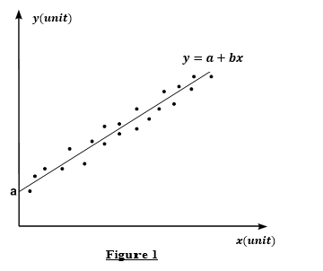
Knowing that we have n measurements performed in practical work, then the values of a and b are given by the formulas:
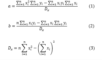
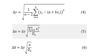
The uncertainties associated with each parameter are given by:
If the linear regression line passes through the origin, we have the equation y = ax of the line ,
in this case a = 0 and we obtain:
-
Experience : A scale repairer wants to replace a defective spring in a scale. The spring must have a stiffness constant
 and a negligible mass. In his workshop, he found a spring of negligible mass but its stiffness constant is unknown.
Using Hook's Law :
 , where F represents the force applied to the spring, k the stiffness constant and d the elongation, he was able to calculate the value of k . As a result, he hung different masses on the spring and measured its elongation. Hook's law simplifies to :
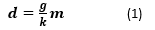
The measurements are reported in the table below.
Questions :
1- By comparing the physical equation (1) with the mathematical formula y = bx , establish the following identifications :
x = , y = , b =
2- Complete the table below :
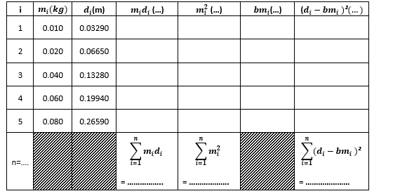
3- Give the numerical values of the following quantities with their corresponding units :
b = ; Δd = ; Δb =
4- On the same graph sheet, represent the experimental points d = f(m), the error bars as well as the line of slope b .
5- Calculate the spring stiffness constant and put it in the form k = (......... ± ….......) .........
6- Can the repairer replace the defective spring ? Explain. We give : g = 9.81 m/s² .
-
I. Goals :
- Highlight the movement of an elementary mechanical system: the oscillating pendulum.
- Determine the spring stiffness constant by two methods: static and dynamic.
- Measure the value of an unknown mass from the spring calibration curve.
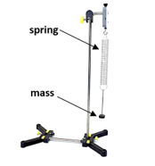
II. USED MATERIAL :
- A support.
- A metal rod.
- A spring of negligible mass
- A box of marked masses.
- A graduated ruler.
- A stopwatch.
- A mass of unknown value.
III. THEORY :
III.1. Static study:
When a mass m is suspended from a spring, the latter lengthens and exerts a force F on the object responsible for its elongation; this force is called spring tension.
The elongation of the spring is noted xeq and is defined by:
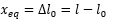
where l0 : is the empty length of the spring
l : the length of the extended spring.
A stiffness spring k , whose mass will be neglected, is suspended vertically by its upper end from a support.
By applying Newton's first law, we have :
At Equilibrium :
From where, by projection on the axis of movement oriented vertically, we obtain: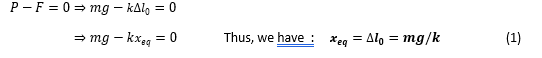
III.2. Dynamic study :
Using the previous spring, in addition to its first elongation Δl0 = xeq due to the clinging mass, we stretch the spring with a distance x (see Fig 2).
By applying Newton's second law, we have :
By projection on the axis of movement oriented vertically, we get : px - Fx = ax
Using the relations :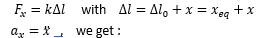
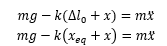
Using the relation (1), we obtain the differential equation of the oscillatory movement.

We can thus determine the expression of the period of the pendulum:
Physically, the period represents the time of one oscillation.
IV. expErimental PROCEDURE:
IV.1. Static study:
1. Start by hanging the spring from the horizontal rod.
2. Attach the ruler so you can take precise measurements.
3. Measure the empty length l0 of the spring.
4. Then you must first suspend the weight rack to be able to place the masses on it.
5. Different known masses (m ) of increasing values (see the table on the TP-sheet) are attached to the spring.
At equilibrium, measure the corresponding elongations (X = xeq ), taking into account the mass of the weight rack.
For each mass, take a minimum of three measurements (each student will take one measurement).
Record your results in the table.
6. To preserve the spring, you must unhook the mass directly after performing the measurement.
Never leave masses attached to the spring!!
7. On a millimeter sheet, draw the calibration curve of the spring X = f(m).
IV.2. Determination of the unknown mass of a body :
We want to determine the unknown mass m of a body from the calibration curve of the spring, for this :
1. Take the device used previously and put the unknown mass to the spring.
2. Measure the elongation X of the spring.
3. Use the spring calibration curve to determine the value of the mass m.
IV.3.Dynamic study :1. Resume the previous device. Attach a known mass m to the spring.
2. Stretch the spring (taking it away from its equilibrium position) a small distance, perfectly vertically, then let go of the mass without initial velocity.
3. Let the mass oscillate and measure the period of the oscillations T (read and carefully follow the measurement instructions on the sheet hung in the laboratory).
4. For each mass, take a minimum of three measurements (Each student will take one measurement).
5. Change mass and follow the same steps. Fill in the measurement table on the TP-sheet.
6. On a millimeter sheet, draw the calibration curve of the spring T2 = f(m)
-
I. GOALS :
- Study the variation of the position of a body, moving on an inclined plane, as a function of time.
- Experimental calculation of the earth's gravitational constant g.
- The calculation of the dynamic coefficient of friction µd .
- The calculation of the static coefficient of friction µs .
II. USED MATERIAL :
- A carriage whose mass m is labeled above.
- An inclined plane of length L = 100 cm.
- A friction block.
- Two optical forks.
- A graduated ruler.
- A digital stopwatch
III. THEORY :
III.1. Movement without friction :
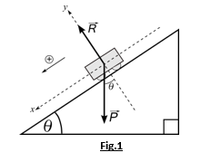
A carriage of mass m slides on an inclined plane that makes an angle with the horizontal plane (see Fig.1).
The fundamental principle of dynamics (FPD), neglecting the effects of plane friction, allows us to write:
The projection on the axis of movement x, gives us :

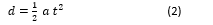
The equation of motion of the carriage can be written in the form :
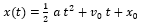
Hence, the expression of the distance d traveled by this trolley, for an
initial speed of zero (v0 = 0) is :
III.2. Movement with friction :
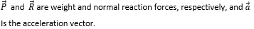
The carriage is now replaced by a friction block. This block is released, without initial speed, from the top of the inclined plane (see Fig.2). The application of FPD principle gives us:
f being the frictional force which is added in this case and a' is the acceleration vector.
Projecting equation (3) onto the x axis, we get:

µd is the dynamic coefficient of friction.
The projection of equation (3) on the axis, gives us :

The equation of motion of the carriage can be written in the form:
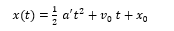
Hence the expression of the distance traveled by this block, for an initial speed of zero ( v0 =0) is :
IV. EXPERIMENTAL PROCEDURE
IV.1. Movement without friction :
In this part, we vary the distance between the two optical forks and we measure the time necessary for the carriage to travel this distance, taking an initial speed of zero.
1. Set the angle of inclination of the plane to 5°.
2. Place the carriage on the plane, so that its cursor is at the limit of the beam of the optical fork. This is the device that starts the stopwatch. If this instruction is not respected, the results will be falsified by the non-zero initial speed of the carriage when the stopwatch is started.
3. For different distances d of increasing values between the two optical forks (see the table in the TP-sheet), measure the corresponding times t. For each distance, take a minimum of three measurements (each student will take one measurement). When the carriage cursor crosses the beam of the second optical fork, the stopwatch stops and it displays the time elapsed for crossing this distance. Record your results in the measurement table.
4. On a millimeter sheet, draw the requested curve.
IV.2. Movement with friction :
IV.2.1. Determination of the dynamic coefficient of friction :
1. Consider the previously used device.
2. Set the angle of inclination of the plane to 20°.
3. Replace the carriage with the friction block.
4. Put the block on the side that contains a single face of felt.
5. The block must be placed on the plane, so that its cursor is at the limit of the beam of the optical fork.
6. Drop the block with no initial velocity. Measure the duration (time) of the movement for the different distances between the two optical forks (see the table in the TP-sheet). Record your results in the measurement table.
7. On a millimeter sheet, draw the required curve.
IV.2.2. Determination of the coefficient of static friction :
1. Take the previously used device.
2. Set the angle of inclination of the plane to 0°.
3. Increase the angle of the incline until the block slides. Note the value of the angle.
4. Calculate the coefficient of static friction.
V. THEORETICAL QUESTIONS (IMPORTANT) :
1. Determine the expression of the acceleration for the movement without friction (case III.1.) of the carriage depending on the earth's acceleration g .
2. Determine the expression of the acceleration for the movement with friction (case III.2.) of the carriage depending on the earth's acceleration and the coefficient of dynamic friction µd .
2. Determine the expression for the coefficient of static friction µs depending on the angle of the inclined plane .
-
FIRST PART: FREE FALL
I. GOALS :
- The study of the motion of a ball dropped without initial velocity in the gravitational field.
- The experimental determination of the acceleration of gravity g.- Study of the effect of the mass on the value of the acceleration g.
II. USED MATERIAL :
- Two balls of different masses.
- A vertical rod which supports at its upper end an horizontal arm.
- An electronic counter.
- A ruler graduated in millimeters.
III. THEORY :
The relationship of distance versus time and the initial velocity of a body in free fall motion is given by the relation :
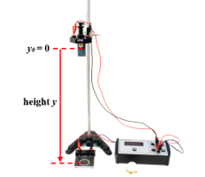
If we fix the origin of the heights at the starting point of the body in free fall, i.e. h0 = 0 (figure above) with zero initial velocity v0 = 0 , the previous relation can be written in the form :

IV. EXPERIMENTAL PROCEDURE :
1. There is a vertical rod which supports at its upper end an horizontal arm.
2. At the free end of the horizontal arm, a mass m is held by a trigger between the tip and the slide by which it triggers a mechanical contact.
3. As soon as the mass is released with the trigger, the mechanical contact is cut and the electronic counter starts up.
4. The mass falls in free fall on the plate which will stop the counter. This system then allows us to measure the time t that the mass takes to travel a vertical distance h.
5. The experimental work consists in measuring the time t for several vertical distances h. The time t is taken using a digital meter.
6. For the measurement of h, use a ruler graduated in millimeters.
IV.1. Experience 1 : Follow the experimental procedure described above, using the ground metal ball m1. Fill in the table found in the technical sheet.
IV.2. Experience 2 : Repeat the previous experiment using the mass plastic ball m2.
Remarks : -The distance h is measured between the lower end of the ball and the plate.
To have good measurements and for the same height, take the average of at least two time measurements.
SECOND PART : TWO-DIMENSIONAL BALLISTIC MOTION
I. GOALS :
- The examination of the effect of the firing angle on the range.
- The determination of the initial velocity of a parabolic falling projectile.
II. USED MATERIAL :
- Mini launcher
- Stainless metal ball
- Carbon paper
- White paper
- Decameter
III. THEORY : The range is the horizontal distance, x, between the muzzle of the mini-shooter and the impact point of the falling ball. :
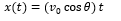
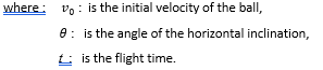
In the vertical direction, where the force of gravity applies, the vertical position y(t) is expressed by :
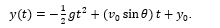
By taking y0 = 0, the point of fall, corresponding to the return of the projectile to the initial vertical position, will be :

Two solutions exist :
The first solution corresponds to the initial position and the second solution thus determines the range. By introducing in the equation of the horizontal position, we obtain :

IV. EXPERIMENTAL PROCEDURE :
1. Choose on the device (mini-launcher) the same release point (to have the same initial speed) and this by placing the ball in the mini-launcher. Place it in the third position indicated on the device One click corresponds to the 1st position, two clicks to the 2nd position and three clicks to the 3rd position.
2. Adjust the angle of the mini launcher to zero degrees (0°) as well as the height of the mini-launcher. The opening of the mini launcher must be at the same level as the table.
3. Place on the table a white sheet above which we will place a 2nd sheet of carbon paper. This allows you to leave a mark when the ball hits the table.
4. Change the shooting angles and measure the range using the decameter.
Theoretical question : Are there two different launch angles giving the same range?
If yes explain. -
I. GOALS :
- Highlight the movement of an elementary mechanical system: the simple pendulum.
- Study the influence of different parameters such as length and mass on the proper period of a simple pendulum.
- Visualize the oscillatory motion and calculate experimentally the value of the earth's acceleration.
II. IMPORTANT :
- The protractor must be properly fixed to the horizontal rod to minimize errors on the angle.
- The ruler must be fixed to a nut and using the brackets located on the ruler, the length of the wire can be measured without too much difficulty.
- Reading on graduated devices such as the ruler or the protractor must be done perpendicular to the device.
- It must be ensured that the movement of the simple pendulum is indeed a swinging movement in a plane. There shouldn't be swings in all directions.
III. USED MATERIEL :
- An adjustable foot on which a rod is fixed horizontally.
- Two balls, considered dimensionless, of masses m1 and m2 ( m1 ≠ m2).
- A graduated ruler of length l=1m .
- An inextensible wire.
IV.THEORY :
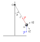
The simple pendulum is made by suspending a ball of mass from an inextensible wire of length , attached to a bracket by its upper end. The ball is moved slightly away from its equilibrium position (amplitude less than 10°) then released.
According to the figure opposite and by applying the fundamental principle of dynamics,
we obtain :
T, P, and m represent respectively the tension of the wire, the weight of the mass suspended on the wire and the acceleration of the pendulum.
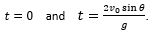
By projecting onto the tangential axis oriented towards the unitary vector ur, we find the equation of motion :
θ.., l and g represent respectively the angular acceleration of the pendulum, the length of the wire and the acceleration of earth's gravity.
Knowing that for low amplitudes, we have sin θ ≈ θ, thus we obtain :

which can be written in the form :

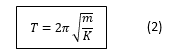
with ω = g/l and like T= 2π/ω then we get the simple period formula :
V. EXPERIMENTAL PROCEDURE:
V-1. Influence of the length of the wire on the period
In this part, we try to verify the influence of the length of the wire on the period of the movement. We start by suspending the ball at the gallows, then, the length of the wire is varied. For each of the lengths considered, the ball is slightly moved away from its equilibrium position then it is released without initial speed. Then, we measure the period of the movement of the pendulum using the stopwatch. Finally, we draw l = f(t2) on a millimeter paper.
V-2. Influence of the mass of the pendulum on the period
In this part, we want to verify the influence of the mass of the ball on the period of the movement. We replace the first mass ball by a second mass ball . We do the same measurements as for the first part then we draw the graph l = f(t2) on a millimeter paper.
-
-
-