PRACTICAL WORK OF PHYSICS (MECHANICS)
| Site: | Campus Numérique UABT |
| Cours: | TP PHYSIQUE 1 (Pratical Work in Mechanics) |
| Livre: | PRACTICAL WORK OF PHYSICS (MECHANICS) |
| Imprimé par: | Visiteur anonyme |
| Date: | dimanche 21 juin 2026, 05:34 |
1. GENERAL RECOMMENDATIONS
ORGANISATION
- A physics (mechanics) practical work PW is scheduled once a fortnight for each group.
- The practical works are performed in ascending order. Example: a student who does PW n°3 in the first session will do PW n°4 in the following session.
- Any justified absence will be made up for in a catch-up session scheduled by the same teacher.
- The justification must be approved by the vice-dean of pedagogy within 48 hours following the absence.
- In case of delay in submitting the justification to the responsible of the matter (more than a week after the absence), the student will have a zero.
- Any unjustified absence will be penalized with a zero.
DISCIPLINE IN THE LABORATORY
A student who comes to physics laboratory must:
- Behaves as a respectful and conscientious student.
- Comes on time (no delay) to the practical session.
- Puts on a white apron.
- Stores stools under benches before going out.
- Has prepared his manipulations (students will be questioned and marked accordingly).
- Brings:
- Scientific calculator.
- Necessary equipment to draw graphs (pencil, eraser, 30cm ruler, millimeter sheets, etc.)
- No exchange of equipment (calculator, pencils, etc.) between students will be tolerated.
- The use of the mobile phone is strictly prohibited even to use it as a calculator.
REPORTS
- The practical work session is reserved for the manipulation and exploitation of the results.
- The curves must be drawn in pencil on an entire graph sheet (millimeter paper).
- Reports should be :
- Written, properly, on practical work sheets provided by the teacher.
- Given individually to the teacher at the end of the session.
- The marks will be provided to students by the responsible teachers fifteen (15) days after the submission of the reports.
2. REMINDER ON THE LINEAR REGRESSION METHOD
We use the linear regression method only when the absolute uncertainty on \( x \) is \( ( \Delta x \approx 0 ) \) negligible and the absolute uncertainty on is constant \( ( \Delta y = cste ) \) .
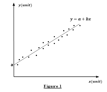
This method consists in drawing the best possible straight line of equation \( y=a+bx \) which passes as close as possible to all the experimental points, as illustrated in figure 1.
\( b \) represents the slope of the regression line while is the ordinate at the origin.
Knowing that we have \( n \) measurements performed in practical work, then the values of \( a \) and \( b \) are given by the formulas:
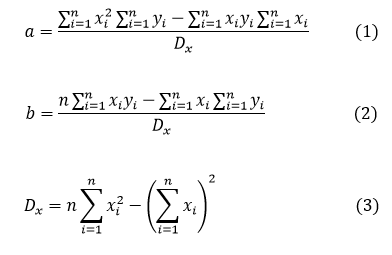
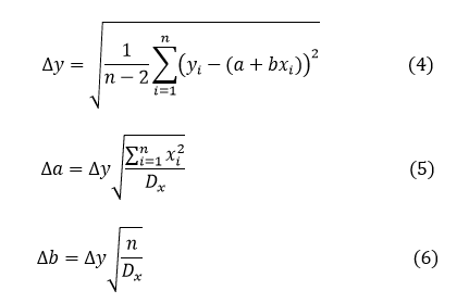
The uncertainties associated with each parameter are given by:
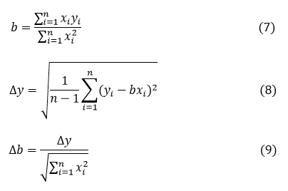
If the linear regression line passes through the origin, we have the equation of the line \( y=bx \), in this case \(a=0\) and we obtain:
3. PW 1: INTRODUCTION TO PHYSICS PRACTICAL WORK
Experience
A scale repairer wants to replace a defective spring in a scale. The spring must have a stiffness constant \( k=(3.00 \pm 0.05) N/m \) and a negligible mass. In his workshop, he found a spring of negligible mass but its stiffness constant is unknown.
Using Hook's Law : \( F=k \times d \) , where \( F \) represents the force applied to the spring, \( k \) the stiffness constant and \( d \) the elongation, he was able to calculate the value of \( k \) . As a result, he hung different masses on the spring and measured its elongation. Hook's law simplifies to :
\( d= \frac{g}{k} m \) (1)
The measurements are reported in the table below.
Questions
- By comparing the physical equation (1) with the mathematical formula \( y=bx \) , establish the following identifications :
\( x= .....................\), \( y= ..................... \) , \( b= ..................... \) - Complete the table below :
- Give the numerical values of the following quantities with their corresponding units :
\( b= .................... \) , \( \Delta d=.................... \) , \( \Delta b=.................... \) . - On the same graph sheet, represent the experimental points \( d=f(m) \), the error bars as well as the line of slope \(b\).
- Calculate the spring stiffness constant and put it in the form \( k=(............. \pm .............) .... \).
- Can the repairer replace the defective spring ? Explain. We give : \(g = 9.81 m/s^2 \).
| i | \( m_i (kg) \) | \( d_i(m) \) | \( m_i d_i (…) \) | \( m_i^2 (…) \) | \( bm_i(…) \) | \( (d_i-bm_i )^2(…) \) |
|---|---|---|---|---|---|---|
| 1 | 0.010 | 0.03290 | ||||
| 2 | 0.020 | 0.06650 | ||||
| 3 | 0.040 | 0.13280 | ||||
| 4 | 0.060 | 0.19940 | ||||
| 5 | 0.080 | 0.26590 | ||||
| \( n=... \) |
\( \sum_{i=1}^{n} m_i d_i \) \(= ....................\) |
\( \sum_{i=1}^{n} m_i^2 \) \(= ....................\) |
\( \sum_{i=1}^{n} (d_i-bm_i )^2 \) \(= ....................\) |
4. PW2 : STATIC AND DYNAMIC STUDIES OF THE OSCILLATING PENDULUM
1. Goals
- Highlight the movement of an elementary mechanical system: the oscillating pendulum.
- Determine the spring stiffness constant by two methods: static and dynamic.
- Measure the value of an unknown mass from the spring calibration curve.
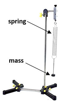
2. Used Material
|
|
|---|
3. Theory
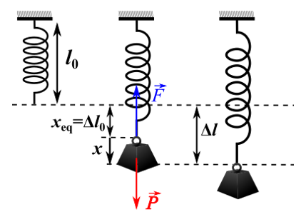
3.1. Static studyWhen a mass \( m \) is suspended from a spring, the latter lengthens and exerts a force \( \vec{F} \) on the object responsible for its elongation; this force is called spring tension.
The elongation of the spring is noted \(x_{eq} \) and is defined by: \(x_{eq} \ = \Delta l_0 = l - l_0\)
where:
- \( l_0 \) is the empty length of the spring
- \( l \) is the length of the extended spring.
A stiffness spring \( k \), whose mass will be neglected, is suspended vertically by its upper end from a support.
By applying Newton's first law, we have :
At Equilibrium : \( \vec{P} + \vec{F}=\vec{0} \) with \( P = mg \) and \( F = k \Delta l_0 =k x_{eq} \)
From where, by projection on the axis of movement oriented vertically, we obtain:
\( P-F=0 \Rightarrow mg-k \Delta l_0 =0 \Rightarrow mg-k x_{eq} =0 \)
Thus, we have :
\( x_{eq}=\Delta l_0 = mg/k \) (1)
3.2. Dynamic studyUsing the previous spring, in addition to its first elongation due to the clinging mass, we stretch the spring with a distance (see the figure above).
By applying Newton's second law, we have : \( \vec{P} + \vec{F}=m\vec{a} \) where (\( \vec{a} \) is the acceleration vector).
By projection on the axis of movement oriented vertically, we get : \(p_x - F_x=a_x\)
Using the relations : \(F_x = k \Delta l \) with \(\Delta l =\Delta l_0 +x = x_{eq} +x \) and \( a_x =\ddot{a} \), we get:
\(mg-k(\Delta l_0 + x ) = m \ddot{x} \)
\(mg-k(\Delta x_{eq} + x ) = m \ddot{x} \)
Using the relation (1), we obtain the differential equation of the oscillatory movement: \( \ddot{x} +\frac{k}{m}x=0 \)with : \( \omega^2=\frac{k}{m} \) and \( \omega =\frac{2\pi}{T} \)
- \(\omega\) : The pulsation
- \(T\) : The period
We can thus determine the expression of the
period of the pendulum:
\( T=2\pi \sqrt{\frac{m}{k}} \) (2)
4. Experimental Procedure
4.1. Static Study
- Start by hanging the spring from the horizontal rod.
- Attach the ruler so you can take precise measurements.
- Measure the empty length \(l_0\) of the spring.
- Then you must first suspend the weight rack to be able to place the masses on it.
- Different known masses (\(m\)) of increasing values (see the table on the PW-sheet) are attached to the spring:
- At equilibrium, measure the corresponding elongations (\(X=x_{eq}\)), taking into account the mass of the weight rack.
- For each mass, take a minimum of three measurements (each student will take one measurement).
- Record your results in the table.
- To preserve the spring, you must unhook the mass directly after performing the measurement. Never leave masses attached to the spring!!.
- On a millimeter sheet, draw the calibration curve of the spring \(x_{eq}=f(m) \).
4.2.Determination of the Unknown Mass of a body
We want to determine the unknown mass \(m\) of a body from the calibration curve of the spring, for this :
- Take the device used previously and put the unknown mass to the spring.
- Measure the elongation \(x_{eq} \) of the spring.
- Use the spring calibration curve to determine the value of the mass\(m \).
4.3.Dynamic Study
- Resume the previous device. Attach a known mass \(m\) to the spring.
- Stretch the spring (taking it away from its equilibrium position) a small distance \(x\), perfectly vertically, then let go of the mass without initial velocity.
- Let the mass oscillate and measure the period of the oscillations \(T\) (read and carefully follow the measurement instructions on the sheet hung in the laboratory).
- For each mass, take a minimum of three measurements (Each student will take one measurement).
- Fill in the measurement table on the PW-sheet.
- On a millimeter sheet, draw the calibration curve of the spring \(T^2=f(m) \)